The problem of extracting useful information from noisy data arises in many domains such as signal processing, wireless sensor networks, and autonomous vehicles. Kalman filtering is a classical approach to solving this problem, and it is now being applied to computer systems problems such as energy management in processors.
This series of blog posts is based on a tutorial on Kalman filtering written for computer systems researchers. This post focuses on applications in which the noisy data are scalar values like temperature. The next one shows how these ideas can be used for state estimation in linear systems. The final one considers applications in which the noisy data are vectors.
A data fusion problem
Suppose we have two instruments for measuring the temperature of a CPU core. If these instruments report different values, as is likely, how can these values be combined to produce a good estimate of the core temperature? This is an example of a data fusion problem.
To address this problem quantitatively, we must specify the noise or error model that explains why the temperature reported by an instrument may be different from the actual core temperature. We’ll make two reasonable assumptions, one about each instrument and one about the relationship between different instruments.
The first assumption is that measurement errors are random and not systematic; intuitively, this means that even if the core temperature is held constant, an instrument may return a different value each time a measurement is made but these values will be clustered around the actual core temperature. Formally, estimates from a given instrument are random samples from a distribution whose (unknown) mean μ is the actual core temperature.

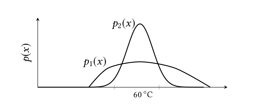
Figure 1: Using distributions to model uncertainty.
Figure 1 shows distributions for two instruments, both centered around 60° C. When the core temperature changes, the distributions shift to the new mean but we assume that their shape remains the same. Therefore the variance of a distribution, which is a measure of its spread, is fixed, and can be used to quantify our confidence in that instrument: the larger the variance, the less our confidence in that instrument. Distributions need not be Gaussian; we assume only that we know the variance of each distribution, and write xi: pi~(σi2) to mean that xi is a random sample from a distribution pi with variance σi2.
The second assumption is that while measurements from each instrument may fluctuate around the actual core temperature, fluctuations in different instruments are unrelated. Formally, the expectation E[(x1-μ)(x2-μ)] = 0. This expectation is called the covariance between x1 and x2, and if it is zero, the variables x1 and x2 are said to be uncorrelated.
Kalman filtering
One obvious solution to our data fusion problem is to discard the measurement from the first instrument, which has higher variance, since we have less confidence in its measurement. Another solution is to take the average of the measurements x1 and x2, using the formula 0.5*x1 + 0.5x2.
Both of these are examples of what statisticians call unbiased linear estimators, whose general form for our problem is yα(x1,x2) = (1-α)*x1 + α*x2 where α is a parameter (in the first solution, α is 1, while in the second one, α is 0.5). The term unbiased refers to the fact that the mean of yα is μ, which is the mean of both x1 and x2.
Is there an “optimal” value of α? Since confidence is inversely proportional to variance, the optimal value of α should minimize the variance of yα. It is easy to show that if x1 and x2 are uncorrelated, the variance of yα is a linear combination of the variances of x1 and x2: σy2(α) = (1-α)2 * σ12 + α2*σ22. Differentiating this with respect to α and setting the derivative to zero, we find that the variance is minimized when α = σ12 ⁄ (σ12 + σ22).
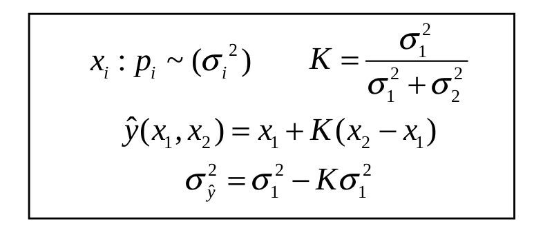
This value of α is called the Kalman gain K. Substituting it into the expressions for yα and σy2, we can write the optimal unbiased linear estimator, denoted by ŷ(x1, x2), and its variance, in terms of K as shown in Figure 2.

Figure 2: Optimal unbiased linear estimator.
Fusing many measurements
To fuse measurements from three or more instruments, we can compute an optimal unbiased estimator that is a weighted sum of n pairwise-uncorrelated measurements. However, there is a simpler way: just as a set of numbers can be added by keeping a running sum and adding the numbers one at a time to this running sum, we can fuse any number of measurements by keeping a “running estimate” and fusing measurements with this running estimate one at a time, updating the value of the running estimate and its variance by using the equations in Figure 2. It can be shown that the output of this running estimator is the same as the result obtained by simultaneously fusing all measurements.
This result is important because in many applications, measurements arrive from different instruments over some period of time. Instead storing all of them and performing one big calculation at the end, we can fuse them “on-line” as they arrive, reducing storage and processing time. This was essential for the use of Kalman filtering in the Apollo space program since computers back then had very little storage and computational capacity.
Final remarks
Kalman filtering tells us that contrary to what we might think intuitively, it is better not to discard noisy measurements from low-confidence instruments because when weighted properly, these measurements can contribute to reducing uncertainty in the overall estimate. In the next post, we show how these ideas can be used for state estimation in linear systems, which is the usual context in which Kalman filtering is presented.
About the Authors: Yan Pei is a graduate student in the CS department at the University of Texas at Austin. Swarnendu Biswas is a post-doctoral research associate in the Institute for Computational Engineering and Science (ICES) at the University of Texas at Austin. Don Fussell is the chair of the CS Department at the University of Texas at Austin. Keshav Pingali (pingali@cs.utexas.edu) is a professor in the CS department and ICES at the University of Texas at Austin.
Disclaimer: These posts are written by individual contributors to share their thoughts on the Computer Architecture Today blog for the benefit of the community. Any views or opinions represented in this blog are personal, belong solely to the blog author and do not represent those of ACM SIGARCH or its parent organization, ACM.


