Uncertainty in Computation and Its Relevance to Computer Architecture
I have recently been thinking about uncertainty in general and uncertainty in computations in particular. It got me thinking about several questions: can uncertainty in computations be exposed above the ISA boundary just like floating-point arithmetic in the IEEE 754 standard and interval arithmetic in IEEE 1788? Would exposing uncertainty handling at the ISA level be a sensible thing to do? What would an ability to handle uncertainty in computations mean for applications? Can we study how uncertainty propagates through some well-known computer architecture benchmark to get some intuition for what it might mean to support uncertainty in computation either at the ISA level or below it in a microarchitecture? And what exactly is uncertainty in the first place? In this post, I’ll look at some of the existing and possible avenues for computer architecture research relating to uncertainty in computation, using a well-known small benchmark as a working example. In a subsequent post, I’ll dive deeper into some existing and possible future paths for computer architects in computation with uncertainty.
There is an interesting recent paper from Manousakis et al. that looked at tracking uncertainty in large-scale server workloads where the computation can be represented as a directed acyclic graph (DAG) and where the execution is implemented by first applying an idempotent function to the DAG and then aggregating the results of that function in a second step (i.e., a MapReduce computation). Reading the work from Manousakis et al. and also recalling the work from Bornholt, Mytkowitz, and McKinley, I thought it would be interesting to pick a self-contained computational task and to track how uncertainty propagates through it using two of the methods available for doing so. My goal is to use this as a kind of mental scaffolding from which to explore how some of these ideas might be implemented in computer architectures and system software. In this first part of two posts, I will describe one such application, a serial version of the blackscholes application from the PARSEC benchmark suite. I picked blackscholes for three reasons: First, it is a microbenchmark which many people in the computer architecture community are familiar with. Second, it has parameters for which we can quantify uncertainty, in the form of an empirical distribution. Third, I hadn’t (at the time) read the original paper by Black and Scholes introducing the model and it seemed like it would be a fun read. Before diving into the Black-Scholes model, its analytic solution, its implementation in the blackscholes benchmark, and how uncertainty propagates through the analytic solution (and its implementation as a program), I’ll first clarify what I (and many others) usually mean when we refer to uncertainty.
Uncertainty in Numbers
Numbers in computing systems are typically either unsigned integers, signed integers, or approximate real numbers in a floating-point representation such as IEEE 754. When the numbers in question are the result of, say, a measurement, the individual values we store and perform computation with are usually the result of multiple instances of the outcome of measuring some quantity with the quantity nominally unchanging. For example, most sensor integrated circuits provide a facility for performing a configurable amount of integration or averaging. This averaging is usually activated with the objective of reducing noise under the assumption that the noise is unimodal (e.g., additive Gaussian noise). An example of averaging that almost everyone has witnessed is that implicitly performed by the image sensor in your camera. The slower the shutter speed (e.g., 1/50s versus 1/4000s), the longer it is averaging the image of the scene on the pixels in the image sensor. A photographer (directly or indirectly) picks the shutter speed and as a result indicates the duration during which they assume the scene is unchanging. At any such shutter speed setting, if you were to repeatedly read (and reset) the values of the camera sensor pixels during the duration when the shutter was open, you could do the integration or averaging in software and you could then also use the data that you were computing the average from to quantify the uncertainty in the pixel measurements.
The true underlying quantity we are attempting to quantify with a measurement is usually referred to as the measurand. The spread across the multiple measurements when the measurand is nominally unchanging is one form of measurement uncertainty. Such uncertainty due to variation in values for a (nominally) fixed measurand is usually referred to as aleatoric uncertainty. We might also have aleatoric uncertainty when we take multiple measurements at the same time using different measurement instruments. It is also possible to have uncertainty in a quantity simply because you have no (or insufficient) information about it. This form of uncertainty is often referred to as epistemic uncertainty. For example, when training a neural network, you start off with high epistemic uncertainty about the weights needed to give good prediction accuracy.
Numeric Computation and Black-Scholes
I will use a concrete application program (written in C), to illustrate how uncertainty in an input parameter leads to uncertainty in the program’s output. The PARSEC blackscholes benchmark, which I will use in the examples below, implements equations corresponding to the solution of the PDE described by the Black-Scholes-Merton model. Black-Scholes-Merton is a theoretical model for assigning a price to a financial instrument which gives the holder of the instrument a right to buy or sell some asset within some specified timeframe. These financial instruments are called options. When they give the holder the right to buy the asset in question, they are more specifically referred to as call options. When they give the holder of the instrument the right to sell the asset under consideration, they are referred to as put options.
The Black-Scholes-Merton model is a second-order partial differential equation. Let s be the price of the asset in question (assumed to follow a log-normal distribution with standard deviation σ over some window of time) and let V be the price of the option on that asset. Let r be the market’s interest rate, for bonds perceived to be risk-free (such as US Treasury bonds). Then, the Black-Scholes-Merton model is:

The Black-Scholes-Merton model was derived based on the insight that the expected return on a hedged position must be equal to the return on a riskless asset such as US treasury bonds. The derivation by Black and Scholes assumed that the distribution of the stock price in continuous time has a variance proportional to the square of the stock price. Under certain assumptions and for the variant of the options where the holder of the option can only exercise the option on a specific date (so-called European options), it is possible to derive explicit closed-form equations for the price of the put options (p(s,t)) and call options (c(s, t)). Let T be the date of maturity of the (European-style) option and let k be the price at which the holder of the option chooses to exercise the option (the so-called strike price). Let N be the cumulative distribution function of the Gaussian distribution. The closed-form analytic equation for the call option price is then

The equation for the put option is similar and so I’ll leave it out since I only use examples of call options next. The main takeaway message is that you have some expression that involves the natural logarithm of the ratio of the asset price s to the strike price k, the square of the volatility σ, and so on. If any of these parameters are uncertain, we would like to know how that uncertainty affects the uncertainty of the computed value c(s, t), given that we are taking squares, square roots, ratios, and so on.
These are the equations which the PARSEC blackscholes benchmark implements and are what I will use for studying how uncertainty propagates through the blackscholes benchmark. I will focus in particular on how uncertainty in the parameter σ in the explicit closed-form equations for the put and call option prices, which is itself a measurement of the uncertainty in the asset price, s, leads to uncertainty in the computed price for a call or put option. The method I will use to study this idea is basic statistical sampling on the distribution of σ and plugging those samples into the equations for p(s, t) and c(s, t) to obtain a distribution of call and put prices.
Uncertainty in Black-Scholes Call- and Put-Option Computation
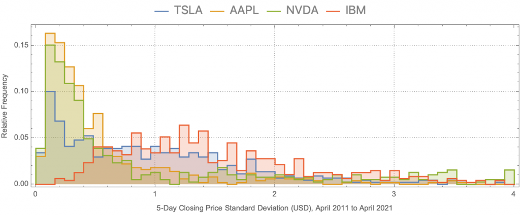
The plot below shows the empirical distributions of standard deviation across closing prices of non-overlapping 5-day sequences, for four stocks (AAPL, NVDA, TSLA, and IBM), over the last 10 years (with 252 trading days per year). The closing price is (obviously) discretized at the granularity of a day which violates the continuous random variable assumption of the derivation of the Black-Scholes model, but closing-price granularity is the finest granularity of historical stock data I have access to.

Statistical Sampling (Monte Carlo) Evaluation of blackscholes Computation
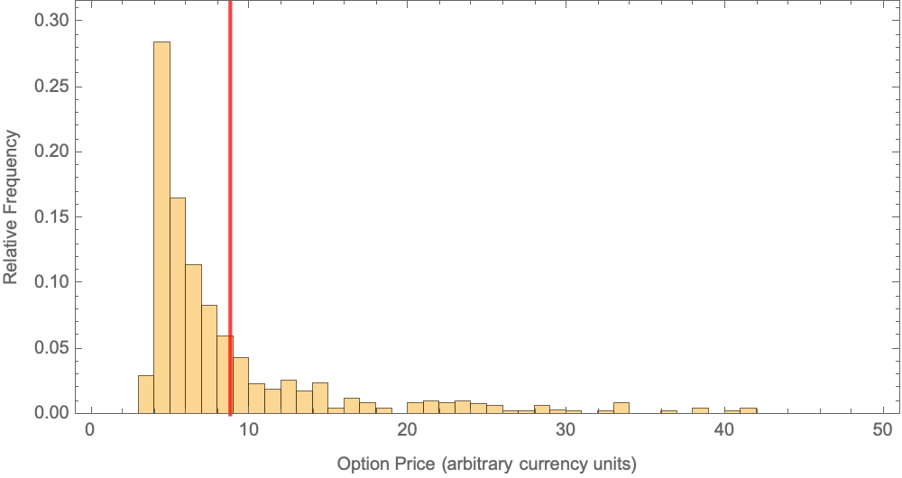
Given the distribution of σ for one of the assets above, we can repeatedly evaluate the closed-form equations for the call or put option price, effectively a Monte Carlo evaluation of the blackscholes benchmark, for a distribution of values of the σ (volatility) parameter. The plot below shows the result of statistical sampling evaluation (i.e., Monte Carlo) of the blackscholes call option price across a distribution of volatility parameter values. The results in the plot below are for an asset spot price of 42, a strike price of 40, a risk-free interest of 10%, a dividend rate of 0%, a time to maturity of 6 months, and volatility as a distribution based on the empirical distribution for stock AAPL in Figure 1. (The foregoing prices are all in arbitrary currency units since the PARSEC blackscholes benchmark does not specify currency units in the example benchmark parameters it provides.) Uncertainty in the volatility (σ) unsurprisingly leads to a distribution in the computed option price. Because of the form of the distribution, it is misleading to look simply at the average value of the result distribution (red marker in the plot).

Statistical Sampling Computations Can Be Cumbersome
The statistical sampling evaluation of blackscholes is cumbersome. For the plot above, I ran the blackscholes benchmark a few thousand times, each time using a value for σ drawn from the empirical distribution of σ for the stock AAPL in Figure 1 and using the remaining parameters as given by a fixed PARSEC benchmark input configuration for blackscholes.
Rather than statistical sampling in this way, the work of Manousakis et al. uses an approximation for propagating uncertainty, represented by a variance, through an expression. The technique, which I will refer to as the linear uncertainty propagation approximation, in a nutshell is an expression for the variance of a function in terms of the variances of its parameters and the partial derivatives of the function with respect to those parameters. (The technique is based on a Taylor series expansion of the function through which we want to propagate uncertainty). Using this method, we would first reduce the volatility distribution in the first figure above to the mean (1.61672) and its standard deviation (22.372). We would then apply the uncertainty propagation approximation to the call option price equation implemented in blackscholes and also listed as the function c(s, t) above. The result would give us c(s, t) = 19.3253 with an uncertainty of 337. Again, these values are in arbitrary currency units since the PARSEC blackscholes benchmark does not specify currency units in the example benchmark parameters it provides.
How Can Computer Architectures Make This Easier or Faster?
In the follow-on post, I will explore some of the potential directions for computer architecture and systems software research for dealing with uncertainty throughout the computing system stack, from sensors, to data storage and filesystems, to computer architectures for processing uncertainty (and whether that even makes sense), and more. I will then tie all these ideas together by looking at how uncertainty in a time-varying signal’s samples affect the outputs of a challenging signal processing algorithm (independent component analysis).
About the Author: Phillip Stanley-Marbell is an Associate Professor in the Department of Engineering at the University of Cambridge where he leads the Physical Computation Laboratory and a Faculty Fellow at the Alan Turing Institute where he co-leads the Interest Group on AI in Resource- and Data-Constrained Environments. His research focuses on investigating methods to use properties of physical systems to improve the efficiency of computation on data from nature.
Disclaimer: These posts are written by individual contributors to share their thoughts on the Computer Architecture Today blog for the benefit of the community. Any views or opinions represented in this blog are personal, belong solely to the blog author and do not represent those of ACM SIGARCH or its parent organization, ACM.


