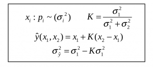
This is the second of a multi-part post that introduces Kalman filtering in an accessible way to computer systems researchers. In the previous post, we described how two noisy estimates of a scalar quantity such as temperature can be fused using the optimal linear unbiased estimator shown in Figure 1. The only assumptions are that (i) we know the variance σi of each estimate xi and (ii) the estimates are uncorrelated.*

Figure 1: Optimal unbiased linear estimator for fusing two noisy estimates.
State estimation in dynamical systems
In this post, we describe how this estimator can be used for state estimation in a discrete-time dynamical system, which is a system whose state evolves at discrete time-steps in response to a control input. At each step, we need an accurate estimate of the state to determine what control input to provide.
One solution is to use a model of the system. For linear systems, this is usually a formula xt+1 = f*xt + b*ut, which computes xt+1, the predicted state at time (t+1), using a linear combination of xt, the state at time t, and ut, the control input applied in the interval [t,t+1). In this formula, f and b are constants determined by the physics of the system (they can even be values that can change at each time-step but we’ll keep it simple). This equation is called a predictor, and in theory, given the initial state x0, we can use it to estimate the state at any time-step. In practice, the initial state and control inputs may not be known exactly and the model may not be completely accurate, so the computed and actual states may diverge unacceptably over time.
Another solution is to use an instrument to measure the state of the dynamical system at each time step, but these measurements may be noisy.
This is where we can use Kalman filtering: if the uncertain state estimate from the predictor and the noisy state measurement from the instrument are not correlated and we know their variances, we can use the equations in Figure 1 to fuse them to produce a more accurate estimate of the state. This fused state estimate is used to determine how to control the system at that time-step, and it is fed back to the predictor formula to perform state estimation for the next time step.

Figure 2: State estimation in a linear dynamical system using Kalman filtering.
Drilling down
To keep all these estimates straight, it is useful to introduce some terminology and notation. The estimate produced by the predictor is called the a priori estimate and is denoted by xt+1|t : intuitively, it is the estimate of the state at time t+1 given the information we have at time t. The measurement at time t+1 is denoted by zt+1. The result of fusing these estimates is called the a posteriori estimate and is denoted by xt+1|t+1.
Figure 2 shows the dataflow diagram of the computation. Each edge in this diagram is labeled with an estimate whose variance is shown in parentheses. The predictor box contains the “application-specific” code that uses the system model to compute the a priori state estimate and its variance. The measurement fusion box is just an instantiation of the generic equations of Figure 2 that fuses the a priori estimate from the predictor with the measurement to produce the a posteriori estimate. To complete the description, we note the following.
- The estimate of the initial state is x0 and its variance is σ0|02.
- Uncertainty in the system model and control inputs is represented by introducing a zero-mean noise term q into the state evolution equation as follows: xt+1 = f*xt + b*ut + q. The variance of q is denoted by σq2 and q is assumed to be uncorrelated with xt|t. Some easy math shows that σt+1|t2 = f2*σt|t2 + σq2. Intuitively, the uncertainty in the a priori estimate comes partly from uncertainty in the a posteriori estimate at the previous step and partly from the model.
- The measurement is assumed to be uncorrelated to the a priori estimate, and its variance is σz2.
Remarks
In the next post, we consider the case when estimates are vectors, such as the position and speed of a spacecraft. The math is more complicated but the good news is that the results in the last two posts can be extended to this case just by replacing variances with covariance matrices. If you have used Kalman filtering in computer architecture applications, we would like to hear from you in the comments.
* In the previous post, we assumed for simplicity of exposition that the means of the estimates were the same, but that assumption is not required by the estimator in Figure 1.
About the Authors: Yan Pei is a graduate student in the CS department at the University of Texas at Austin. Swarnendu Biswas is a post-doctoral research associate in the Institute for Computational Engineering and Science (ICES) at the University of Texas at Austin. Don Fussell is the chair of the CS Department at the University of Texas at Austin. Keshav Pingali (pingali@cs.utexas.edu) is a professor in the CS department and ICES at the University of Texas at Austin.
Disclaimer: These posts are written by individual contributors to share their thoughts on the Computer Architecture Today blog for the benefit of the community. Any views or opinions represented in this blog are personal, belong solely to the blog author and do not represent those of ACM SIGARCH or its parent organization, ACM.


